
在执行books['Date'].at[i] = start + timedelta(days=i)时会报错
unsupported type for timedelta days component: numpy.int64
最终修改为books['Date'].at[i] = start + timedelta(days=int(i))可以正常运行

在执行books['Date'].at[i] = start + timedelta(days=i)时会报错
unsupported type for timedelta days component: numpy.int64
最终修改为books['Date'].at[i] = start + timedelta(days=int(i))可以正常运行
# 蔓藤教育,pandas操作excel的行和列等
import pandas as pd
# 创建一个序列,在pandas中,数据帧DataFram和序列Series是最基本的数据结构
# pandas中的序列的第一种方法,由python中的字典改变而来
d = {'x': 100, 'y': 200, 'z': 300}
print(d)
s1 = pd.Series(d)
# 创建序列的第二种方法
L1 = [100, 200, 300]
L2 = ['x', 'y', 'z']
s2 = pd.Series(L1, index=L2)
#s2.to_excel('output3.xlsx', header=None)
# 序列在excel中可能是行,也可能是列,根据传递进DataFrame中序列的方法不同,在excel中呈现行或列不同
s3 = pd.Series([1, 2, 3], index=[1, 2, 3], name='A')
s4 = pd.Series([10, 20, 30], index=[1, 2, 3], name='B')
s5 = pd.Series([100, 200, 300], index=[1, 2, 3], name='C')
# 当以字典形式将序列传递进数据帧时,在excel中以列呈现
# 创建ExcelWriter对象实现向excel中不同sheet中追加写入内容,否则会被覆盖
writer = pd.ExcelWriter('output.xlsx')
df = pd.DataFrame({s3.name: s3, s4.name: s4, s5.name: s5})
#df.to_excel('output3.xlsx', sheet_name='sheet1')
df.to_excel(writer, sheet_name='字典传入为列')
# 当以列表List形式传入时,以行的形式存在
df1 = pd.DataFrame([s3, s4, s5])
#df1.to_excel('output3.xlsx', sheet_name='sheet2')
df1.to_excel(writer, sheet_name='列表传入为行')
writer.save()
import pandas as pd
笔记,不错。
不能直接贴屏?!
图片要用文件上传模式,一般。
一、涉及知识点
1、pandas读取已经存在的Excel文件
2、涉及的BIF操作:
df=pd.read_excel('F:/sdf/sdf/output.xlsx',header=None)
pd.to_excel('F:/sdf/sdf/output1.xlsx')
df.shape
df.columns
df.header(5)
df.tail(5)
二、问题点
1、读取xls文件异常(xlrd.biffh.XLRDError: Unsupported format, or corrupt file: Expected BOF record; found b'Test Tim')
原因:源文件损坏,或者格式有问题(虽然是以.xls结尾,但实际上内容格式有问题的)
一、涉及知识点
1、Excel和pandas创建excel格式的数据源
2、数据格式有很多,常见的如下:CSV文件、数据库表格、文件格式(Excel、PDF、Word等)、HTML文件、JSON文件、文本文件、XML文件
二、遇到的问题及原因
1、pandas库找不到(AttributeError: module 'pandas' has no attribute 'DataFrame')
原因:1)未安装pandas库
2)pycharm中解释器配置错误(项目多时需要配置虚拟环境,每个虚拟环境中挂载的库都不一样,pycharm的setting中会有默认的配置,需检查是否错误)
import pandas as pd
people=pd.dread_excle('C:/Temp/people.xlsx')
print(people.shape)
print(people.columns)
print('==================')
print(people.tail(3))
import pandas as pd
df=pd.DataFrame[{'ID':[1,2,3],'Name':['Tim','Victor','N}]
df.to_excel('C:/Temp/output.xlsx')
print('Done!')
d
饿,TIM老师的这个方程其实是可以化简的,也不是很复杂
import pandas as pd
import numpy as np

# def get_circumcircle_area(l,h):
#     r = np.sqrt(l**2+h**2)/2
#     return r**2*np.pi

# def get_circumcircle_area(l,h):
#     return np.pi*(l**2+h**2)/4
#
# def wrapper(row):
#      return get_circumcircle_area(row['Length'],row['Height'])

rects = pd.read_excel('D:/Temp/Rectangles.xlsx',index_col='ID')
rects['CA'] = rects.apply(lambda row:np.pi*(row['Length']**2+row['Height']**2)/4,axis=1)

print(rects)
这样的话一行就可以了
https://www.jianshu.com/p/2d49cb87626b
对于group详细的解析
字符串前加f是用于格式化字符串的,
print(f'#{row.ID}student{row.Name}has an invalid score{row.Score}.')
就相当于
print('# %d student{row.Name}has an invalid score %s.' % (row.ID,row.Score))
具体上网搜一下python 字符串格式化的三种方法就好了
students['2017'].sort_values(ascending=True).plot.pie(fontsize=6,startangle=-270)
可以用在乱序的情况
老师资料里matplotlib里面的代码应该用的不是同一个文件了,要改一下

import numpy as np
import pandas as pd
import matplotlib.pyplot as plt

students = pd.read_excel('D:/Temp/Students10.xlsx')
students.sort_values(by='2017', inplace=True, ascending=False)
students.index = range(0, len(students))
print(students)

bar_width = 0.7
x_pos = np.arange(len(students) * 2, step=2)
plt.bar(x_pos, students['2016'], color='orange', width=bar_width)
plt.bar(x_pos + bar_width, students['2017'], color='red', width=bar_width)

plt.xticks(x_pos + bar_width / 2, students['Field'], rotation='90')
plt.title('International Student by Field', fontsize=16)
plt.xlabel('Field')
plt.ylabel('Number')
plt.tight_layout()
plt.show()
matplotlib感觉和matlab很像
products
def age_18_to_30(a):
return 18<=a<=30
def level_a(s):
return 85<=s<=100
students=pd.read_excel('C:/temp/students.xlsx',index_col='ID')
students.loc[students['Age'].apply(age_18_to_30)].loc[students['Score'].apply(level_a)]
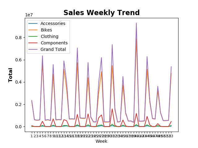
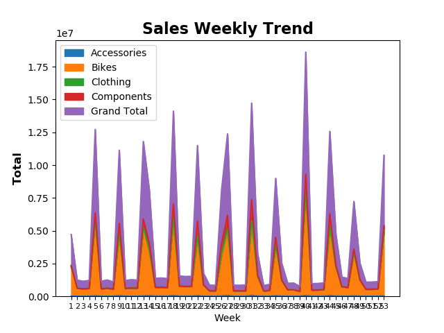
任务13:绘制折线趋势图、叠加区域图
!!!!本课下载下来的excel附件名字是Order.xlsx. 编辑代码时注意修改!!!
本课代码:
import pandas as pd
import matplotlib.pyplot as plt
weeks = pd.read_excel('C:/Temp/Orders.xlsx', index_col='Week')
print(weeks)
print(weeks.columns)
#weeks.plot.area(y=['Accessories', 'Bikes', 'Clothing', 'Components', 'Grand Total'])
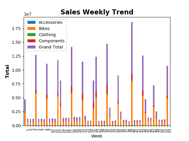
weeks.plot.bar(y=['Accessories', 'Bikes', 'Clothing', 'Components', 'Grand Total'], stacked=True)
plt.title('Sales Weekly Trend', fontsize=16, fontweight='bold')
plt.ylabel('Total', fontsize=12, fontweight='bold')
plt.xticks(weeks.index, fontsize=8)
plt.show()
打印结果:
       Accessories         Bikes      ...         Components   Grand Total
Week                                  ...
1      9939.465500  2.258337e+06      ...       7.872110e+04  2.356639e+06
2     12626.660000  6.005350e+05      ...       0.000000e+00  6.204234e+05
3     14414.950000  5.547708e+05      ...       0.000000e+00  5.759616e+05
4     12924.580000  5.892557e+05      ...       0.000000e+00  6.083717e+05
5     40443.498516  5.749222e+06      ...       4.709014e+05  6.360041e+06
6     13735.460000  5.539423e+05      ...       0.000000e+00  5.753385e+05
7     13588.800000  6.053847e+05      ...       0.000000e+00  6.247596e+05
8     13997.810000  5.320056e+05      ...       0.000000e+00  5.526938e+05
9     52392.263204  4.701389e+06      ...       6.852023e+05  5.567191e+06
10    14276.640000  5.815496e+05      ...       0.000000e+00  6.037474e+05
11    13584.320000  6.169319e+05      ...       0.000000e+00  6.372021e+05
12    14128.770000  5.985606e+05      ...       0.000000e+00  6.204505e+05
13    34372.148628  5.154563e+06      ...       6.173474e+05  5.899177e+06
14    58097.712659  3.361458e+06      ...       5.296900e+05  4.041540e+06
15    16287.020000  6.655744e+05      ...       0.000000e+00  6.894546e+05
16    15990.960000  6.749113e+05      ...       0.000000e+00  6.991723e+05
17    15120.710000  6.581411e+05      ...       0.000000e+00  6.795171e+05
18    67753.596201  5.739679e+06      ...       1.091392e+06  7.059584e+06
19    15416.040000  7.537814e+05      ...       0.000000e+00  7.770648e+05
20    16113.010000  7.323520e+05      ...       0.000000e+00  7.571492e+05
21    15903.150000  7.380932e+05      ...       0.000000e+00  7.620668e+05
22    57090.139277  4.388471e+06      ...       1.137457e+06  5.746683e+06
23    11900.146000  8.310402e+05      ...       3.152596e+04  8.824418e+05
24    11336.820000  4.095025e+05      ...       0.000000e+00  4.251703e+05
25    10573.210000  4.065446e+05      ...       0.000000e+00  4.232483e+05
26    29376.532664  3.101888e+06      ...       7.994845e+05  4.039316e+06
27    72003.211677  4.932875e+06      ...       1.043760e+06  6.191153e+06
28    11621.900000  4.086479e+05      ...       0.000000e+00  4.258483e+05
29    11640.460000  4.056193e+05      ...       0.000000e+00  4.225788e+05
30    12359.920000  4.156482e+05      ...       0.000000e+00  4.325679e+05
31    81276.364307  5.475372e+06      ...       1.593068e+06  7.363333e+06
32    15208.996500  1.494933e+06      ...       1.025128e+05  1.623856e+06
33    13187.100000  3.938290e+05      ...       0.000000e+00  4.135150e+05
34    13046.980000  4.383911e+05      ...       0.000000e+00  4.571066e+05
35    50187.449516  3.732927e+06      ...       5.842441e+05  4.495606e+06
36    15063.164000  1.173016e+06      ...       6.180437e+04  1.260751e+06
37    11505.920000  4.814773e+05      ...       0.000000e+00  4.985188e+05
38    13170.670000  4.883039e+05      ...       0.000000e+00  5.066807e+05
39    11278.600000  3.675468e+05      ...       0.000000e+00  3.845985e+05
40    70170.520320  7.878476e+06      ...       1.177747e+06  9.303972e+06
41    12441.460000  4.658615e+05      ...       0.000000e+00  4.834701e+05
42    12924.950000  4.715758e+05      ...       0.000000e+00  4.907546e+05
43    13314.310000  4.931541e+05      ...       0.000000e+00  5.127108e+05
44    62745.172581  5.156642e+06      ...       9.100149e+05  6.286165e+06
45    19630.003108  2.199453e+06      ...       1.478740e+05  2.381990e+06
46    14822.180000  7.092621e+05      ...       0.000000e+00  7.304781e+05
47    13728.300000  6.623922e+05      ...       0.000000e+00  6.830832e+05
48    36075.469500  3.240381e+06      ...       2.592590e+05  3.616344e+06
49    13642.418500  1.227307e+06      ...       2.369806e+04  1.273325e+06
50    12388.980000  5.217178e+05      ...       0.000000e+00  5.419306e+05
51    12852.400000  5.264518e+05      ...       0.000000e+00  5.455141e+05
52    13085.680000  5.412245e+05      ...       0.000000e+00  5.604452e+05
53    31315.891268  4.790804e+06      ...       4.568886e+05  5.375680e+06

[53 rows x 5 columns]
Index(['Accessories', 'Bikes', 'Clothing', 'Components', 'Grand Total'], dtype='object')
Series序列类似于dictionary
生成一个序列
d={'x':100,'y':200,'z':300}#字典/键值对
print(d.keys())#所有键
print(d.values())#所有值
print(d['x'])#具体一个值
s1=pd.Series(d)#字典转为序列
-----------------------------------
第二种创建序列方法
s1=pd.Series([100,200,300],index=['x','y','z'])
s1=pd.Series(data,index,name)#序列既不是行也不是列
s2=pd.Series(data,index,name)#序列只有加入DataFrame才能有行和列的区别,而这种区别是建立在加入时的方法不同上:两种加入法:dictonary 或者list
pd.DataFrame({s1.name:s1,s2.name:s2})#以dictonary加入当作列
pd.DataFrame([s1,s2])
pd.DataFrame(list)#以list加入当作行
index的作用:
对齐原则
有共同值则对齐,没有共同值的位置给一个NaN空
--------------------------------------
下节学习:使用Series进行快速填充